PyTorch + ANI + MD

PyTorch provides nice utilities for differentiation. ANI provides some interatomic potentials trained on some neural networks. Molecular Dynamics might be an interesting combination

Some basic pytorch functionality, a 1-D spring

Pytorch replicates a lot of numpy functionality, and we can build python functions that take pytorch tensors as input

import torch
import matplotlib.pyplot as plt

x = torch.ones((2,2), requires_grad=True)

A simple quadratic function

def sq_function(x):
    return x**2

Since we have an array of 1s, the square won’t look very interesting…

foo = sq_function(x)

foo

tensor([[1., 1.],
        [1., 1.]], grad_fn=<PowBackward0>)

More interstingly, we can compute the gradient of this function.

To compute the gradient, the value/function needs to be a scalar, but this scalar could be computed from a bunch of other functions stemming from some independent variables (our tensor x). In this case, our final scalar looks like this, $ Y = x_0^2 + x_1^2 + x_2^2 + x_3^2 $. Taking the gradient means taking 4 partial derivatives for each input. Fortunately, the equation is simple to compute each partial derivative, $ \frac{\partial Y}{\partial x_i} = 2*x_i $, where $i = [0,4)$. Since this is an array of 1s, each partial derivative evaluates to 2

torch.autograd.grad(foo.sum(), x)

(tensor([[2., 2.],
         [2., 2.]]),)

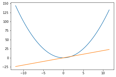
We’ve evaluated the function and its gradient at just one point, but we can use some numpy-esque functions to evaluate the square-function and its gradient at a range of points.

Yup, looks right to me

some_xvals = torch.arange(-12., 12., step=0.5, requires_grad=True)
some_yvals = sq_function(some_xvals)
fig, ax = plt.subplots(1,1)
ax.plot(some_xvals.detach().numpy(), some_yvals.detach().numpy())
ax.plot(some_xvals.detach().numpy(), 
       torch.autograd.grad(some_yvals.sum(), some_xvals)[0])

[<matplotlib.lines.Line2D at 0x7f9c907aa910>]

Slightly more book-keeping, 3x 1-D harmonic springs

Define an energy function as the sum of 3 harmonic springs

$ V(x, y, z) = V_x + V_y + V_z = (x-x_0)^2 + (y-y_0)^2 + (z-z_0)^2 $

The gradient, the 3 partial derivatives, are computed as such (being verbose with the chain rule)

$ \frac{\partial V}{\partial X} = 2 *(x-x_0) * 1 $

$\frac{\partial V}{\partial Y} = 2 *(y-y_0) * 1$

$\frac{\partial V}{\partial Z} = 2 *(z-z_0) * 1$

def harmonic_spring_3d(coord, origin=torch.tensor([0,0,0])):
    V_x = (coord[0]-origin[0])**2
    V_y = (coord[1]-origin[1])**2
    V_z = (coord[2]-origin[2])**2
    
    return V_x + V_y + V_z 

We can evaluate the potential energy at 1 point, which involves computing the energy in 3 dimensions.

Our “anchor” will be the origin, and our endpoint will be (1,2,3)

$ 1^2 + 2^2 + 3^2 = 14 $

my_coords = torch.tensor([1.,2.,3.], requires_grad=True)
total_energy = harmonic_spring_3d(my_coords)
total_energy

tensor(14., grad_fn=<AddBackward0>)

Computing the gradient, partial derivatives in each direction, which is simply 2 times the distance in each dimension

$ \nabla \hat V = < 21, 22, 2*3 > = <2,4,6> $

torch.autograd.grad(total_energy, my_coords)

(tensor([2., 4., 6.]),)

More involved: Lennard Jones

The Lennard-Jones potential describes the potential energy between two particles. Not the most accurate potential, but has been decent for a long time now. Some background information on the Lenanrd-Jones potential. For simplicity, assume $\epsilon =1$ and $\sigma=1$ in unitless quantities:

$ V_{LJ} = 4 * ( \frac{1}{r}^{12} - \frac{1}{r}^6) $

$ -\frac{\partial V}{\partial r} = -4 * (-12 * r^{-13} + 6 * r^{-7}) $

def lj(val):
    return 4 * ((1/val)**12 - (1/val)**6)

r_values = torch.arange(0.1, 12., step=0.001, requires_grad=True)

energy = lj(r_values)

forces = -torch.autograd.grad(energy.sum(), r_values)[0]

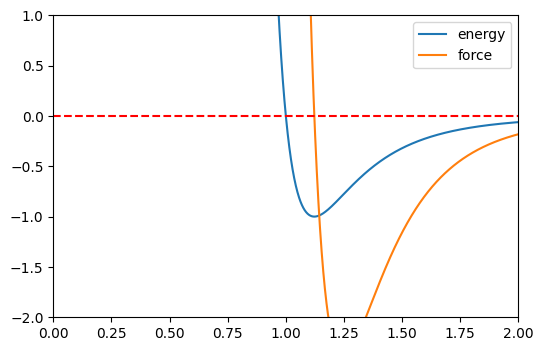
For sanity check, we can confirm that energy reaches a critical point (local minimum) when the force is 0.

Also, this definitely looks like a LJ potential to me

import matplotlib.pyplot as plt

fig, ax = plt.subplots(1,1, dpi=100)
ax.plot(r_values.detach().numpy(), energy.detach().numpy(), label='energy')
ax.plot(r_values.detach().numpy(), forces.detach().numpy(), label='force')
ax.set_ylim([-2,1])
ax.legend()
ax.set_xlim([0,2])
ax.axhline(y=0, color='r', linestyle='--')

<matplotlib.lines.Line2D at 0x7f9d2859b2d0>

Moving to torchani

ANI is an interatomic potential built upon neural networks. Rather than write our own function to evaluate the energy between atoms, maybe we can just use ANI. Since this is pytorch-based, this is still available for autodifferentiation to get the forces

https://github.com/aiqm/torchani

To begin, we have to define our elements (a tensor of atomic numbers). For the molecular mechanics people, each atom is identifiable by its element, and not one of many atom-types.

We have to define the positions (units of Angstrom), which is also a multi-dimensional tensor.

Load the model, specifying to convert the atomic numbers to indices suitable for ANI.

We can compute the energies and forces from the model. The energy comes from the model, but the force is obtained via an autograd call, observing that we are differentiating the sum of the forces, evaluating at the positions

import torchani

elements = torch.tensor([[6, 6]])
positions = torch.tensor([[[3.0, 3.0, 3.0],
                           [3.5, 3.5, 3.5]]], requires_grad=True)

model = torchani.models.ANI2x(periodic_table_index=True)

energy = model((elements, positions)).energies

forces = -1.0 * torch.autograd.grad(energy.sum(), positions)[0]

/home/ayang41/miniconda3/envs/torch37/lib/python3.7/site-packages/torchani/aev.py:195: UserWarning: This overload of nonzero is deprecated:
	nonzero()
Consider using one of the following signatures instead:
	nonzero(*, bool as_tuple) (Triggered internally at  /pytorch/torch/csrc/utils/python_arg_parser.cpp:766.)
  in_cutoff = (distances <= cutoff).nonzero()

energy

tensor([-75.7952], dtype=torch.float64, grad_fn=<AddBackward0>)

forces

tensor([[[-0.4016, -0.4016, -0.4016],
         [ 0.4016,  0.4016,  0.4016]]])

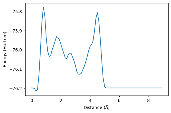
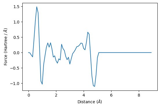
Going a step further, we can try to visualize the interaction potential by evaluating the energy at a variety of distances. We can also do some autodifferentiation to compute the forces.

In this example, we have 2 atoms that share X and Y coordinates, but pull them apart in the Z direction

all_z = torch.arange(3.0, 12.0, step=0.1)
all_energy = []
all_forces = []
for z in all_z:
    # Generate a new set of positions
    positions = torch.tensor([[[3.0, 3.0, 3.0],
                               [3.0, 3.0, z]]], requires_grad=True
                            )
    # Compute energy
    energy = model((elements, positions)).energies
    # Compute force
    forces = -1.0 * torch.autograd.grad(energy.sum(), positions)[0]
    
    # Get the force vector on the first atom
    one_atom_forces = forces[0,0]
    # Compute the magnitude of this force vector
    force_magnitude = torch.sqrt(torch.dot(one_atom_forces, one_atom_forces))
    # Calculate the unit vector for this force vector,
    # although it's a little unnecessary because the only distance is in the
    # z direction
    unit_vector_force = one_atom_forces/force_magnitude
    # Get z-component of force vector
    force_vector_z = unit_vector_force[2]*force_magnitude
    # Some nans will form if the force magnitude is zero, but this
    # is really just a 0 force vector
    if torch.isnan(force_vector_z).any():
        force_vector_z = 0.0
    else:
        force_vector_z = float(force_vector_z.detach().numpy())
    
    # Accumulate
    all_energy.append(float(energy.detach().numpy()))
    all_forces.append(force_vector_z)

Hmmm… this does not resemble the Lennard-Jones potential (or basic chemistry for that matter)

fig, ax = plt.subplots(1,1, dpi=100)
ax.plot(all_z-3, all_energy)
ax.set_xlabel(r"Distance ($\AA$)")
ax.set_ylabel("Energy (Hartree)")

Text(0, 0.5, 'Energy (Hartree)')

fig, ax = plt.subplots(1,1, dpi=100)
ax.plot(all_z-3, all_forces)

ax.set_xlabel(r"Distance ($\AA$)")
ax.set_ylabel("Force (Hartree / $\AA$)")

Text(0, 0.5, 'Force (Hartree / $\\AA$)')

Combinng torchani with some other molecular modeling libraries

We’re going to use mbuild to initialize some particles, mdtraj as a convenient library to hold molecular information, and torchani to calculate some energies. As with the 2-atom potential example, this pentane example is a little fishy, but this code snippet should hopefully serve as a nice framework to combine some open source molecular modeling libraries.

from mbuild.lib.recipes import Alkane

# The mBuild alkane recipe is mainly used to generate 
# some particles and positions
cmpd = Alkane(n=5)

# Convert to mdtraj trajectory out of convenience for atomic numbers
traj = cmpd.to_trajectory()

# Periodic cell, from nm to angstrom
cell = torch.tensor(traj.unitcell_vectors[0]*10)

# We just need atomic numbers
species = torch.tensor([[
    a.element.atomic_number for a in traj.top.atoms
]])

# Make tensor for coordinates
# Since we are differentiating WRT coordinates, we need the
# requires_grad=True
coordinates = torch.tensor(traj.xyz*10, requires_grad=True)

# PBC flag necessary for computing energies with periodic boundaries
pbc = torch.tensor([True, True, True], dtype=torch.bool)

energies = model((species, coordinates), cell=cell, pbc=pbc).energies

forces = -1.0 * (
    torch.autograd.grad(energies.sum(), coordinates)[0]
)

energies

/home/ayang41/miniconda3/envs/torch37/lib/python3.7/site-packages/ipykernel/ipkernel.py:287: DeprecationWarning: `should_run_async` will not call `transform_cell` automatically in the future. Please pass the result to `transformed_cell` argument and any exception that happen during thetransform in `preprocessing_exc_tuple` in IPython 7.17 and above.
  and should_run_async(code)





tensor([-197.1103], dtype=torch.float64, grad_fn=<AddBackward0>)

forces

/home/ayang41/miniconda3/envs/torch37/lib/python3.7/site-packages/ipykernel/ipkernel.py:287: DeprecationWarning: `should_run_async` will not call `transform_cell` automatically in the future. Please pass the result to `transformed_cell` argument and any exception that happen during thetransform in `preprocessing_exc_tuple` in IPython 7.17 and above.
  and should_run_async(code)





tensor([[[ 6.5805e-02,  5.5707e-02,  4.9085e-02],
         [ 1.3603e-03, -2.1826e-02, -1.0588e-02],
         [ 1.5610e-02, -5.9448e-02,  1.4180e-03],
         [-7.4506e-09,  1.1921e-07,  1.1461e-02],
         [-7.2804e-03,  2.5767e-02, -6.2775e-04],
         [ 7.2804e-03, -2.5766e-02, -6.2775e-04],
         [-6.5805e-02, -5.5707e-02,  4.9085e-02],
         [-1.5610e-02,  5.9448e-02,  1.4180e-03],
         [-1.3604e-03,  2.1826e-02, -1.0588e-02],
         [ 6.9919e-02,  1.0938e-01, -4.7381e-02],
         [ 4.2583e-02,  1.5188e-01, -9.1655e-03],
         [-3.5887e-02, -5.4712e-03,  4.6396e-02],
         [ 3.4462e-03,  3.7552e-02, -3.4868e-02],
         [-6.9919e-02, -1.0938e-01, -4.7381e-02],
         [-4.2583e-02, -1.5188e-01, -9.1655e-03],
         [ 3.5887e-02,  5.4712e-03,  4.6396e-02],
         [-3.4462e-03, -3.7552e-02, -3.4868e-02]]])

To be continued …

One might imagine trying to incorporate ANI potentials into MD simulations (which has been done in ASE). However, the torchani-API is general enough that you could use any number of computational chemistry packages to feed into torchani. The output is also general enough you could imagine trying to apply your own integrators and make your own simulation. But… from the weird 2-atom interatomic potentials, some of these methods might require some debugging.

Files and environment can be found here

Reference

Xiang Gao, Farhad Ramezanghorbani, Olexandr Isayev, Justin S. Smith, and Adrian E. Roitberg. TorchANI: A Free and Open Source PyTorch Based Deep Learning Implementation of the ANI Neural Network Potentials. Journal of Chemical Information and Modeling 2020 60 (7), 3408-3415