Big data tools for MD simulation analysis

(Updated 2020-05-15)

Trajectories are sets of coordinates over time. While the act of gathering data and conducting simulations are exhaustively parallelized, some analysis methods are not. Speaking from experience, parallelizing analysis using Python multiprocessing can get very messy if you don’t have a clear idea of how you want to parallelize the analysis, and how exactly you’re going to code it up.

Here, I’m going to attempt to use some parallel librareis for MD trajectory analysis

Some big data tools

Since grad school, I’ve been exposed to a variety of big data tools (Dask, Spark, Rapids), and it’s been a point of interest to test their utility to molecular simulation. Each tool comes with its own sets of advantages and disadvantages, and I encourage everyone to actively try each to see which is most appropriate for the desired application.

• Rapids is very fast, but requires GPUs. Depending on your tech stack and tech constraints, you may or may not have cheap and easy access to sufficient GPUs. Rapids is a little more sensitive to data types than others - but as an amateur, I could be misusing the libraries.
• Spark is fast, but requires some hadoop and Spark knowhow to stand up properly. Many tech stacks and constraints seem to be well-suited for spark applications. Spark scales out well, very flexible with datatypes, and eschews a lot of parallel programming-knowhow. At my own work, some primitive tests have shown that spark outperforms dask for dataframe operations on strings and some ML operations - but as an amateur, there is probably some Dask tuning that could be done
• Dask is also fast, but your mileage may vary. Some tech stacks are suitable for Dask, but cloud resources/tech constraints might make Dask adoption hard. Dask exposes various levels of parallelism, so proper Dask-users will end up learning a lot about parallel computing along the way.

I defer to this pydata video for a Dask, Rapids, Spark comparison

For those like me who are not used to setting up parallel compute

The one thing I will observe as I dabble away on my personal computer - I am neither familiar with setting up a Hadoop cluster nor am I familiar with exposing my WSL to my GPU, and single-node pyspark is not going to useful for the overhead. If given the proper infrastructure and resources, I can use these libraries, but at this moment it would take time for me to set up the resources to properly utilizes Spark or Rapids on my PC. Dask, in my case, seems like the simplest parallel compute library to use. If you’re a grad student or a data scientist unfamiliar with software environments and infrastructure beyond Conda environments, Dask might also be easiest for adoption.

Computing atomic distances from a molecular dynamics simulation

Trivial MD analysis involves looking at each atom within a frame, and not having to look at time correlations from frame to frame. I’m going to use MDTraj to load in a trajectory, and look at distances between atoms in each frame. I’ll do this serial, with just MDTraj, and I’ll do this with using one level of Dask parallelism, Dask delayed

import itertools as it
from pathlib import Path
import numpy as np


import mdtraj
import dask
from dask import delayed
import dask.bag as db

Saving myself the effort of generating my own trajectory, I will use one of the trajectories in MDTraj’s unit tests

path_to_data = Path('/home/ayang41/programs/mdtraj/tests/data')
tip3p_xtc = Path.joinpath(path_to_data/'tip3p_300K_1ATM.xtc')
tip3p_pdb = Path.joinpath(path_to_data/'tip3p_300K_1ATM.pdb')

This trajectory is only 401 frames - parallel analysis incurs too much overhead to be useful. I’m going to artificially lengthen the trajectory out to 1604 frames, where the gain from parallelization will hopefully be more apparent. In reality, most grad students will have many, many more frames to analyze.

traj = mdtraj.load(tip3p_xtc.as_posix(), top=tip3p_pdb.as_posix())
for i in range(2):
    traj = traj.join(traj)
traj

<mdtraj.Trajectory with 1604 frames, 774 atoms, 258 residues, and unitcells at 0x7f9bf4cce150>

Additionally, to load up the computational expense, I’ll look at all pairwise atomic distances in each frame

atom_pairs = [*it.permutations(np.arange(0, traj.n_atoms),2)]

Simple implementation with MDTraj

On my PC with 6 cores, this took about 23 seconds (and also nearly froze my computer).

It should be noted that MDTraj already does a lot of parallelization and acceleration under their hood with some C optimizations. “Simple” in this case, is a user depending on MDTraj’s optimizations

%%time

displacements = mdtraj.compute_displacements(traj, atom_pairs)

CPU times: user 5.94 s, sys: 17.5 s, total: 23.5 s
Wall time: 23.7 s

Combining Dask with MDTraj

Like most parallel computing applications, it’s important to recognize how and what you will be parallelizing/distributing. In this case, we will be distributing our one trajectory across 4 partitions, creating Delayed objects. Each Delayed object isn’t an actual execution - it’s a scheduled operation (like queueing something up in SLURM or PBS).

It helps that mdtraj.Trajectory objects are iterable, so we can easily break up the trajectory into 4 even-sized chunks with some python list comprehensions

%%time
chunksize = int(traj.n_frames/4)
bag = db.from_sequence([traj[chunksize*i: chunksize*(i+1)] for i in range(4)] , npartitions=4)
bunch_of_delayed = bag.to_delayed()

CPU times: user 62.5 ms, sys: 172 ms, total: 234 ms
Wall time: 293 ms

bag

dask.bag<from_sequence, npartitions=4>

bunch_of_delayed

[Delayed(('from_sequence-b688539387c3c167fe82241b18a1670a', 0)),
 Delayed(('from_sequence-b688539387c3c167fe82241b18a1670a', 1)),
 Delayed(('from_sequence-b688539387c3c167fe82241b18a1670a', 2)),
 Delayed(('from_sequence-b688539387c3c167fe82241b18a1670a', 3))]

If we wanted to, we can still pluck out and execute the Delayed objects, and parse the number of atoms in MDTraj-like syntax

bunch_of_delayed[0].compute()[0].n_atoms

774

We can also validate that each Delayed object is computing a quarter of our trajectory

bunch_of_delayed[0].compute(), bunch_of_delayed[1].compute()

([<mdtraj.Trajectory with 401 frames, 774 atoms, 258 residues, and unitcells at 0x7fb555e2df50>],
 [<mdtraj.Trajectory with 401 frames, 774 atoms, 258 residues, and unitcells at 0x7fb2a1a12d10>])

To queue up additional computations, we will take each Delayed object, and add on one additional operation - mdtraj.compute_displacements. Now the delayed objects have two operations - distributing the trajectory and computing the displacements. It’s worth noting that none of these operations involved rewriting MDTraj code or adding function decorators. These MDTraj functions are wrapped using the Delayed objects

Again, the computation has not been performed yet

%%time
all_displacements = [delayed(mdtraj.compute_displacements)(traj[0], atom_pairs) for traj in bunch_of_delayed]
all_displacements

CPU times: user 26.5 s, sys: 2.55 s, total: 29 s
Wall time: 29.2 s





[Delayed('compute_displacements-c1ef5c08-6bb2-4508-8f1a-166000d2cd3e'),
 Delayed('compute_displacements-5a9fd8cd-2993-4c4b-be90-a2523e47c09a'),
 Delayed('compute_displacements-35c48042-fecf-4eb4-adc5-931c097b6e8d'),
 Delayed('compute_displacements-d8699960-98e0-4b74-a320-2b2e1f3870a9')]

If we want to “flush” the queue and run all our Delayed computations, we use Dask to finally compute them.

At this point, the actual calculation took 3min 6s (hey, this is terrible!), but the overhead involved 27 seconds

%%time
displacements = dask.compute(all_displacements)

CPU times: user 17.8 s, sys: 27.9 s, total: 45.7 s
Wall time: 3min 6s

The returned object is 4 different results, and each result is a numpy array 401 x 598302 x 3 (n_frames x n_atompairs x n_spatialdimensions)

len(displacements[0])

4

displacements[0][1].shape

(401, 598302, 3)

Visualizing the dask graph

Spark and Dask both use task graphs to schedule function after function, with Spark doing some implicit optimizations.

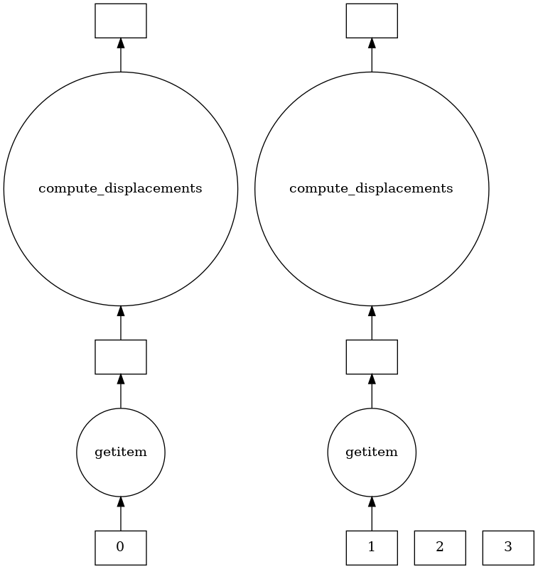
Dask has a nice visualize functionality to show what the task graphs and parallelization look like for two of our Delayed objects

dask.visualize(all_displacements[0:2])

This Dask parallelization slowed the MDTraj operation down! What gives?

MDTraj is very well-optimized, so any attempts to distribute work end up slowing down the array multiplications

We’ll use our own, crude distance function that has no optimizations (and doesn’t obey the minimum image convention)

def crude_distances(traj, atom_pairs):
    all_distances = []
    for frame in traj:
        distances =[]
        for pair in atom_pairs:
            distance = np.sqrt(np.dot(frame.xyz[0, pair[0], :], frame.xyz[0, pair[1], :]))
            distances.append(distance)
        all_distances.append(distances)
    return np.array(all_distances)

%%time
traj = mdtraj.load(tip3p_xtc.as_posix(), top=tip3p_pdb.as_posix())
chunksize = int(traj.n_frames/4)
bag = db.from_sequence([traj[chunksize*i: chunksize*(i+1)] for i in range(4)] , npartitions=4)
bunch_of_delayed = bag.to_delayed()

CPU times: user 125 ms, sys: 0 ns, total: 125 ms
Wall time: 505 ms

atom_pairs = [*it.combinations(np.arange(0,100),2)]

%%time
all_displacements = [delayed(crude_distances)(traj[0], atom_pairs) for traj in bunch_of_delayed]
all_displacements

CPU times: user 156 ms, sys: 46.9 ms, total: 203 ms
Wall time: 169 ms





[Delayed('crude_distances-fb865e6f-232a-4a24-8a37-0b0f6ce13f22'),
 Delayed('crude_distances-438627d2-a181-4127-85a1-1cfbe99f64f6'),
 Delayed('crude_distances-543f6412-6dcc-4a30-922b-2f963e978a5d'),
 Delayed('crude_distances-78883eb2-520e-4c75-9af9-d06b82b746d1')]

%%time
output = dask.compute(all_displacements)

CPU times: user 54.6 s, sys: 1min, total: 1min 55s
Wall time: 1min 7s

%%time

output = crude_distances(traj, atom_pairs)

CPU times: user 1min 28s, sys: 1min 40s, total: 3min 8s
Wall time: 1min 51s

So there was ~47 second speedup from the crude function - that’s a small win.

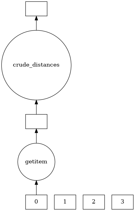
And here’s the task graph for one of the Delayed objects

all_displacements[0].visualize()

Aiming for memory-efficiency

Up until now, we’ve had the whole trajectory loaded into memory prior to any parallelization with Dask. We can use MDTraj’s iterload function to reduce the size of the trajectory, but still pass different chunks around.

As another consideration for parallelization, increasing the number of disk reads will slow down your process, so make sure the gain from parallelization makes it worth it

%%time

delayed_load = db.from_sequence(a for a in mdtraj.iterload(tip3p_xtc.as_posix(), top=tip3p_pdb.as_posix())).to_delayed()

CPU times: user 172 ms, sys: 172 ms, total: 344 ms
Wall time: 312 ms

Confirming that each Delayed object has different frames

delayed_load[0].compute()[0].time, delayed_load[1].compute()[0].time

(array([ 0.,  1.,  2.,  3.,  4.,  5.,  6.,  7.,  8.,  9., 10., 11., 12.,
        13., 14., 15., 16., 17., 18., 19., 20., 21., 22., 23., 24., 25.,
        26., 27., 28., 29., 30., 31., 32., 33., 34., 35., 36., 37., 38.,
        39., 40., 41., 42., 43., 44., 45., 46., 47., 48., 49., 50., 51.,
        52., 53., 54., 55., 56., 57., 58., 59., 60., 61., 62., 63., 64.,
        65., 66., 67., 68., 69., 70., 71., 72., 73., 74., 75., 76., 77.,
        78., 79., 80., 81., 82., 83., 84., 85., 86., 87., 88., 89., 90.,
        91., 92., 93., 94., 95., 96., 97., 98., 99.], dtype=float32),
 array([100., 101., 102., 103., 104., 105., 106., 107., 108., 109., 110.,
        111., 112., 113., 114., 115., 116., 117., 118., 119., 120., 121.,
        122., 123., 124., 125., 126., 127., 128., 129., 130., 131., 132.,
        133., 134., 135., 136., 137., 138., 139., 140., 141., 142., 143.,
        144., 145., 146., 147., 148., 149., 150., 151., 152., 153., 154.,
        155., 156., 157., 158., 159., 160., 161., 162., 163., 164., 165.,
        166., 167., 168., 169., 170., 171., 172., 173., 174., 175., 176.,
        177., 178., 179., 180., 181., 182., 183., 184., 185., 186., 187.,
        188., 189., 190., 191., 192., 193., 194., 195., 196., 197., 198.,
        199.], dtype=float32))

%%time
all_displacements = [delayed(crude_distances)(traj[0], atom_pairs) for traj in delayed_load]
all_displacements

CPU times: user 188 ms, sys: 93.8 ms, total: 281 ms
Wall time: 294 ms





[Delayed('crude_distances-d2f8fad8-663a-41b4-a97c-9277cc086fba'),
 Delayed('crude_distances-4a9116d4-96f0-4c35-bca1-0525622976c8'),
 Delayed('crude_distances-6aa987e4-0e71-462f-9293-55e6deed1425'),
 Delayed('crude_distances-cd230400-cf2f-4ad9-9cc7-ab573848e397'),
 Delayed('crude_distances-627969a1-2726-4f7e-87a9-7a97665c46b0')]

Still ~40 second gain with the crude distance calculation with Dask

%%time
out = dask.compute(all_displacements)

CPU times: user 52.1 s, sys: 1min 3s, total: 1min 55s
Wall time: 1min 10s

%%time
all_displacements = []
for traj in mdtraj.iterload(tip3p_xtc.as_posix(), top=tip3p_pdb.as_posix()):
    all_displacements.append(crude_distances(traj, atom_pairs))

CPU times: user 1min 26s, sys: 1min 46s, total: 3min 13s
Wall time: 1min 51s

atom_pairs = [*it.combinations(np.arange(0, traj.n_atoms),2)]

delayed_load = db.from_sequence(a for a in mdtraj.iterload(tip3p_xtc.as_posix(), top=tip3p_pdb.as_posix())).to_delayed()

%%time
all_displacements = [delayed(mdtraj.compute_displacements)(traj[0], atom_pairs) for traj in delayed_load]

CPU times: user 15.6 s, sys: 688 ms, total: 16.3 s
Wall time: 16.4 s

%%time
out = dask.compute(all_displacements)

CPU times: user 7.98 s, sys: 938 ms, total: 8.92 s
Wall time: 8.92 s

%%time
all_displacements = []
for traj in mdtraj.iterload(tip3p_xtc.as_posix(), top=tip3p_pdb.as_posix()):
    all_displacements.append(mdtraj.compute_displacements(traj, atom_pairs))

CPU times: user 1.17 s, sys: 1.09 s, total: 2.27 s
Wall time: 2.26 s

Trying Dask distributed

We could try another level of parallelism using Dask’s distributed framework on a single node, but there appear to be Dask distributed issues with WSL.

Regardless, we can still see what happens

from distributed import Client

client = Client()
client

distributed.comm.tcp - WARNING - Could not set timeout on TCP stream: [Errno 92] Protocol not available
distributed.comm.tcp - WARNING - Could not set timeout on TCP stream: [Errno 92] Protocol not available
distributed.comm.tcp - WARNING - Could not set timeout on TCP stream: [Errno 92] Protocol not available
distributed.comm.tcp - WARNING - Could not set timeout on TCP stream: [Errno 92] Protocol not available
distributed.comm.tcp - WARNING - Could not set timeout on TCP stream: [Errno 92] Protocol not available
distributed.comm.tcp - WARNING - Could not set timeout on TCP stream: [Errno 92] Protocol not available
distributed.comm.tcp - WARNING - Could not set timeout on TCP stream: [Errno 92] Protocol not available
distributed.comm.tcp - WARNING - Could not set timeout on TCP stream: [Errno 92] Protocol not available
distributed.comm.tcp - WARNING - Could not set timeout on TCP stream: [Errno 92] Protocol not available

distributed.comm.tcp - WARNING - Could not set timeout on TCP stream: [Errno 92] Protocol not available
distributed.comm.tcp - WARNING - Could not set timeout on TCP stream: [Errno 92] Protocol not available
distributed.comm.tcp - WARNING - Could not set timeout on TCP stream: [Errno 92] Protocol not available

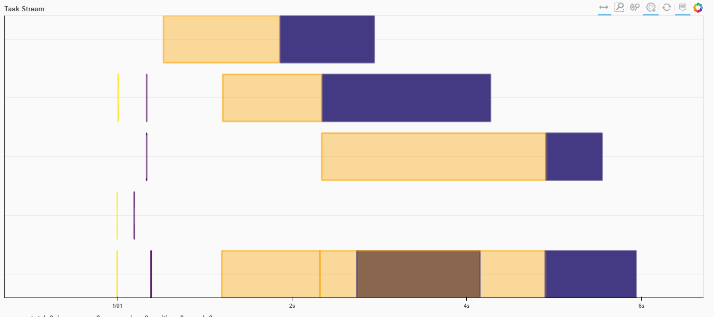
With default settings, we’re working with 3 workers across 6 cores.

We can see from the Dask dashboard that there are certainly concurrent operations, but the yellow operation (disk-read-compute_displacements) is adding a lot of overhead beyond that purple operation (the actual compute_displacements)

%%time
delayed_load = db.from_sequence(a for a in mdtraj.iterload(tip3p_xtc.as_posix(), top=tip3p_pdb.as_posix())).to_delayed()
all_displacements = [delayed(mdtraj.compute_displacements)(traj[0], atom_pairs) for traj in delayed_load]
out = dask.compute(all_displacements)

distributed.comm.tcp - WARNING - Could not set timeout on TCP stream: [Errno 92] Protocol not available
distributed.comm.tcp - WARNING - Could not set timeout on TCP stream: [Errno 92] Protocol not available
distributed.comm.tcp - WARNING - Could not set timeout on TCP stream: [Errno 92] Protocol not available
distributed.comm.tcp - WARNING - Could not set timeout on TCP stream: [Errno 92] Protocol not available
distributed.comm.tcp - WARNING - Could not set timeout on TCP stream: [Errno 92] Protocol not available
distributed.comm.tcp - WARNING - Could not set timeout on TCP stream: [Errno 92] Protocol not available
distributed.comm.tcp - WARNING - Could not set timeout on TCP stream: [Errno 92] Protocol not available
distributed.comm.tcp - WARNING - Could not set timeout on TCP stream: [Errno 92] Protocol not available
distributed.comm.tcp - WARNING - Could not set timeout on TCP stream: [Errno 92] Protocol not available
distributed.comm.tcp - WARNING - Could not set timeout on TCP stream: [Errno 92] Protocol not available
distributed.comm.tcp - WARNING - Could not set timeout on TCP stream: [Errno 92] Protocol not available
distributed.comm.tcp - WARNING - Could not set timeout on TCP stream: [Errno 92] Protocol not available


CPU times: user 37.6 s, sys: 12.4 s, total: 50 s
Wall time: 57.6 s

client.close()
client = Client(processes=False)
client

distributed.comm.tcp - WARNING - Could not set timeout on TCP stream: [Errno 92] Protocol not available
distributed.comm.tcp - WARNING - Could not set timeout on TCP stream: [Errno 92] Protocol not available

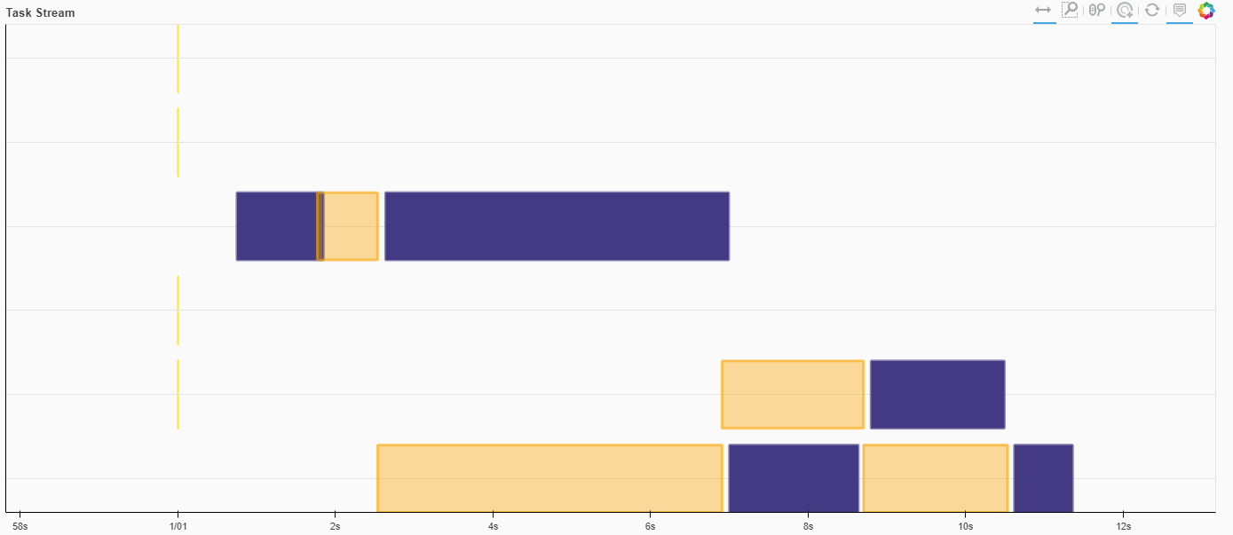
Running all workers on the same process, there’s still some room for multithreading, but the same slow-downs rear their heads

%%time
delayed_load = db.from_sequence(a for a in mdtraj.iterload(tip3p_xtc.as_posix(), top=tip3p_pdb.as_posix())).to_delayed()
all_displacements = [delayed(mdtraj.compute_displacements)(traj[0], atom_pairs) for traj in delayed_load]
out = dask.compute(all_displacements)

distributed.utils_perf - WARNING - full garbage collections took 45% CPU time recently (threshold: 10%)
distributed.utils_perf - WARNING - full garbage collections took 44% CPU time recently (threshold: 10%)
distributed.utils_perf - WARNING - full garbage collections took 44% CPU time recently (threshold: 10%)
distributed.utils_perf - WARNING - full garbage collections took 45% CPU time recently (threshold: 10%)
distributed.utils_perf - WARNING - full garbage collections took 45% CPU time recently (threshold: 10%)
distributed.utils_perf - WARNING - full garbage collections took 46% CPU time recently (threshold: 10%)
distributed.utils_perf - WARNING - full garbage collections took 46% CPU time recently (threshold: 10%)


CPU times: user 51 s, sys: 1.22 s, total: 52.2 s
Wall time: 52.9 s

Takeaways from some Dask tests

The observations here were surprising, but maybe a good lesson before anyone immediately tries to jump into some big data tools

MDTraj is really performant

If you’re able to use MDTraj-optimized functions, use those. If you want to be memory efficient and stream trajectory data, use MDTraj for that; you don’t need to schedule loading different slices of a trajectory with Dask.

An optimized library can beat the bloat of a scheduler

Combining Dask + MDTraj was worse in all cases than just using MDTraj exclusively. Dask’s parallelization didn’t make anything run faster, and Dask’s delayed scheduling didn’t introduce anything better compared to MDTraj’s iterloading. This might be because of multiple reads, communication between workers, or overhead of building out the task scheduler.

If the opportunity, resources, and need exist, optimizing a library can go farther than trying to lump Dask on top of any code. Dask + my-bad-distance-code made things faster than my-bad-distance-code exclusively, but my bad-distance-code was completely devoid of optimization. But throw an optimized library like MDTraj in, and you likely won’t need Dask (or your poorly-written code!).

If you have a particularly unique function you don’t know how to optimize, then it’s time to think about what dask can offer

MDTraj is great because it provides a set of common, optimized functions. For a lot of work in this field, there will be unique analyses that are not common to many MD libraries, and if they are, they may not be optimized. If these two hold true to your particular studies, then your options become

1) Optimize your analysis code. Simplify routines for time and space complexity, reduce for-loops if you can, reduce the amount of read/write operations, write Cython/C/Cuda/compiled code

2) Use a parallel/scheduler framework like Dask

If you’re not a (parallel) programming wiz or lack the time to become one, then option 2 may be for you

It doesn’t help that we’re working with different data

A lot of Dask use-cases and API are built around arrays and dataframes, so there’s already a lot of built-in optimization for those data structures. There may be room to build a Dask-trajectory object that creates room for computational optimization (rather than stringing together a bunch of non-dask operations) that might be able to beat MDTraj

Lastly, the notebook can be found here