NBA defensive schemes
Published:
Team defensive schemes
Does a team’s defensive scheme influence opponents’ shot portfolios? I’m going to be using a different NBA API to query all the games for the 2018-2019 regular season. In each game, I’m going to log each “make” against a team’s defense. For example, Houston makes a 22-ft 3-point shot against Boston, I will log the distance at which Houston scored against Boston.
I’m going to be presenting this as a matrix within a pandas DataFrame, where each row is the defensive team, each column is the offensive team, and each entry is a list of distances for every successful make (excluding free throws). Conveniently, if you look across a row, you’ll be examining that team’s defense against all other teams. Conversely, if you look down a column, you’ll be examiniing that team’s offense against all other teams.
Some caveats to this analysis:
- There are some errors to some game logs, but there are only a few, and those will have a negligible influence since each team plays 82 games anyways.
- Player injuries may influence a team’s defensive/offensive play, but hopefully the team’s tactics still hold.
- The game logs themselves may log each team’s acctions “messily”. If you look at the code, the logic to classify a make involves finding the word ‘make’ and not finding the word ‘free throw’. On top of that, I’m doing some very rudimentary parsing to find the distance of each make.
- Maybe I ought to normalize for pace or opposing team’s “average” offensive skill/behavior, but just histogramming the counts of each make should hopefully be enough to get a sense of a defensive team’s allowed-shot portfolio.
- Because we’re only looking at “makes”, a blocked shot and missed shot are both equally neglected when detecing “makes”, although, in reality, a blocked shot could say more about the defender while a missed shot might say more about the shooter.
WARNING, the cell below takes over an hour to run
from basketball_reference_scraper.constants import TEAM_ABBR_TO_TEAM, TEAM_TO_TEAM_ABBR
from basketball_reference_scraper.seasons import get_schedule
from basketball_reference_scraper.shot_charts import get_shot_chart
from basketball_reference_scraper.pbp import get_pbp
import pandas as pd
from pprint import pprint
import time
start = time.time()

# Each row is the defensive team
# Each column is the offensive team
# Each element is a list of successful makes by the offensive team against the defensive team

TEAMS = ['ATLANTA', 'BOSTON', 'BROOKLYN', 'CHICAGO', 'CHARLOTTE',
        'CLEVELAND', 'DALLAS', 'DENVER', 'DETROIT',
         'GOLDEN STATE', 'HOUSTON', 'INDIANA', 'LA CLIPPERS',
         'LA LAKERS', 'MEMPHIS', 'MIAMI', 'MILWAUKEE', 'MINNESOTA',
         'NEW ORLEANS', 'NEW YORK', 'OKLAHOMA CITY', 'ORLANDO', 'PHILADELPHIA',
         'PHOENIX', 'PORTLAND', 'SACRAMENTO', 'SAN ANTONIO', 'TORONTO',
         'UTAH', 'WASHINGTON']# 'NEW JERSEY NETS',
         #'NEW ORLEANS HORNETS', 'NEW ORLEANS OKLAHOMA CITY HORNETS', 'CHARLOTTE BOBCATS', 'SEATTLE SUPERSONICS', 'VANCOUVER GRIZZLIES']

# Because of how pandas converts dictionaries into dataframes,
# the "first" key is actually the column, while the "second" key is the row
# team_a is defending team, team_b is offending team
shots_dict = {team_a: {team_b:[] for team_b in TEAMS} for team_a in TEAMS}


s = get_schedule(2019, playoffs=False) # Schedule of all games in the 2018-2019 regular season
for i, series in s.iterrows():
    # Get play by play for the given game
    try:
        pbp = get_pbp(series['DATE'],
                    TEAM_TO_TEAM_ABBR[series['HOME'].upper()],
                    TEAM_TO_TEAM_ABBR[series['VISITOR'].upper()])
        teams = series[['HOME', 'VISITOR']] # teams['HOME'], teams['VISITOR']

        # Tidy up strings to format the team name and get the appropriation action
        if "LAKERS" in teams['HOME'].upper():
            home_team = 'LA LAKERS'
            home_actions = pbp['LA LAKERS_ACTION']
        elif "CLIPPERS" in teams['HOME'].upper():
            home_team = 'LA CLIPPERS'
            home_actions = pbp['LA CLIPPERS_ACTION']
        elif "TRAIL BLAZERS" in teams['HOME'].upper():
            home_team = 'PORTLAND'
            home_actions = pbp['PORTLAND_ACTION']
        else:
            home_team = ' '.join(a for a in teams['HOME'].split(' ')[:-1]).upper()
            home_actions = pbp[home_team.upper()+ "_ACTION"]

        if "LAKERS" in teams['VISITOR'].upper():
            visitor_team = 'LA LAKERS'
            visitor_actions = pbp['LA LAKERS_ACTION']
        elif "CLIPPERS" in teams['VISITOR'].upper():
            visitor_team = 'LA CLIPPERS'
            visitor_actions = pbp['LA CLIPPERS_ACTION']
        elif "TRAIL BLAZERS" in teams['VISITOR'].upper():
            visitor_team = 'PORTLAND'
            visitor_actions = pbp['PORTLAND_ACTION']
        else:
            visitor_team = ' '.join(a for a in teams['VISITOR'].split(' ')[:-1]).upper()
            visitor_actions = pbp[visitor_team.upper()+ "_ACTION"]

        # Look at the home team's actions, particularly those on offense
        for offense_action in home_actions[pd.notna(home_actions)]:
            words = offense_action.split(' ')
            success = 'makes' in offense_action and 'free throw' not in offense_action
            if success:
                if 'ft' not in words: # "makes 2-pt layup at rim"
                    shots_dict[home_team][visitor_team].append(0)
                else: # "makes 2-pt jump shot/layup from 3 ft"
                    distance_index = words.index('ft') - 1
                    distance = int(words[distance_index])
                    shots_dict[home_team][visitor_team].append(distance)

        # Look at the visitor team's actions, particularly those on offense
        for offense_action in visitor_actions[pd.notna(visitor_actions)]:
            words = offense_action.split(' ')
            success = 'makes' in offense_action and 'free throw' not in offense_action
            if success:
                if 'ft' not in words: # "makes 2-pt layup at rim"
                    shots_dict[visitor_team][home_team].append(0)
                else: # "makes 2-pt jump shot/layup from 3 ft"
                    distance_index = words.index('ft') - 1
                    distance = int(words[distance_index])
                    shots_dict[visitor_team][home_team].append(distance)
    except AttributeError:
        print(f"Error looking at game {i}")
        continue
end = time.time()
print('Looping took {} seconds'.format(end-start))
df = pd.DataFrame.from_dict(shots_dict)
df.to_pickle('data.pkl')
Looping took 4483.57711315155 seconds
import pandas as pd
df = pd.read_pickle('data.pkl')
# Plotting a team's defense versus other teams
%matplotlib inline
import matplotlib.pyplot as plt
for i, series in df.iterrows():
    fig, ax = plt.subplots(6,5, figsize=(12,10), sharex=True, sharey=True)

    for j, off_team in enumerate(series.index):
        row = j // 5
        col = j % 5
        ax[row, col].hist(series[off_team], bins=[0, 5, 15, 22, 35], density=False)
        ax[row,col].set_ylabel(f"Makes by\n{off_team}")
        ax[row,col].set_xlabel("Distance (ft)")
        ax[row,col].set_xticks([0, 5, 15, 22, 35])
        ax[row,col].set_xticklabels([0, 5, 15, 22, 35])
        ax[row,col].set_ylim([0, 100])

    fig.tight_layout()
    simple_name = '_'.join(a for a in series.name.split(' '))
    fig.savefig(f"{simple_name}_defense.png", transparent=True)
    plt.close(fig)
Worst NBA regular season defenses
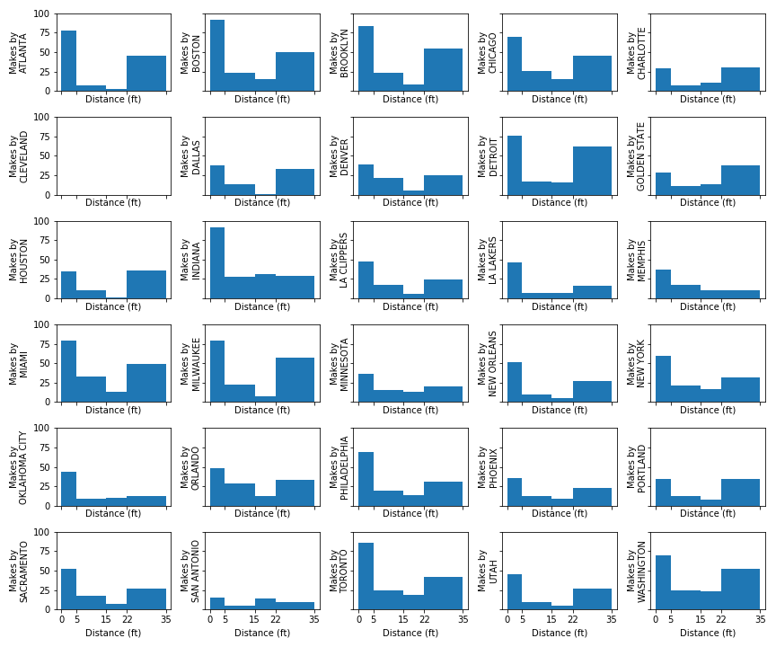
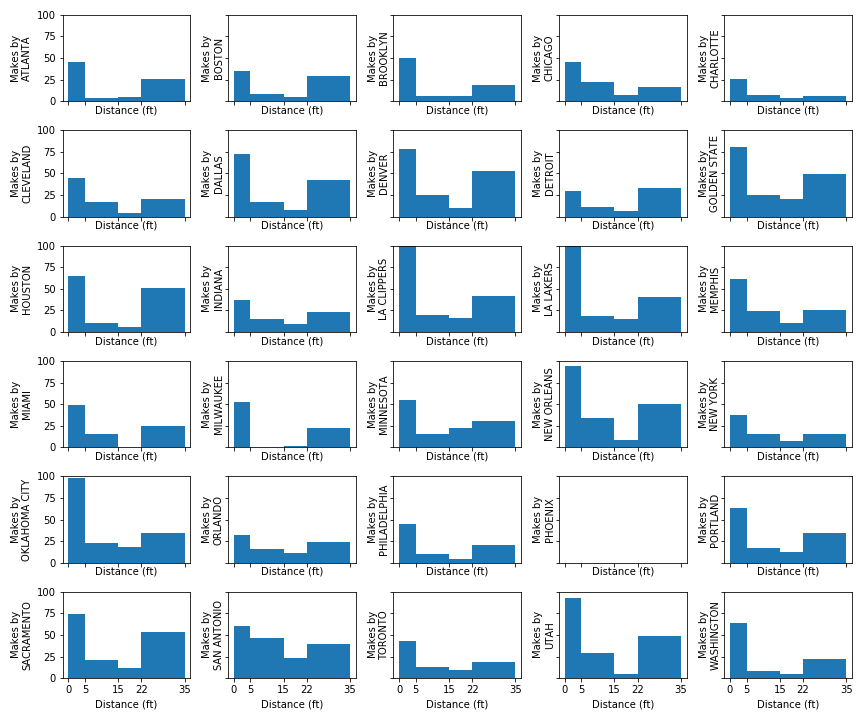
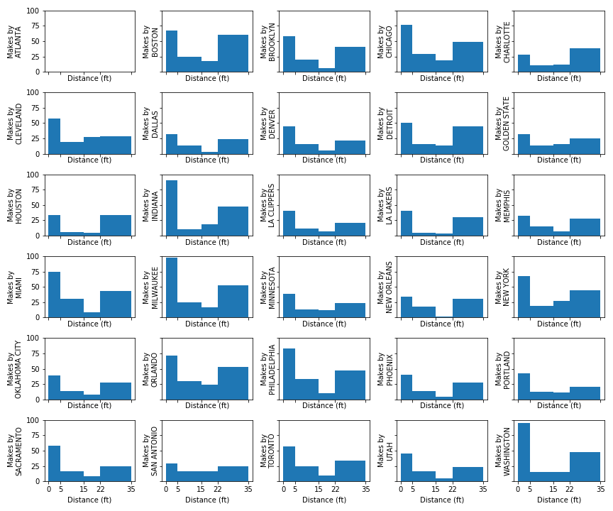
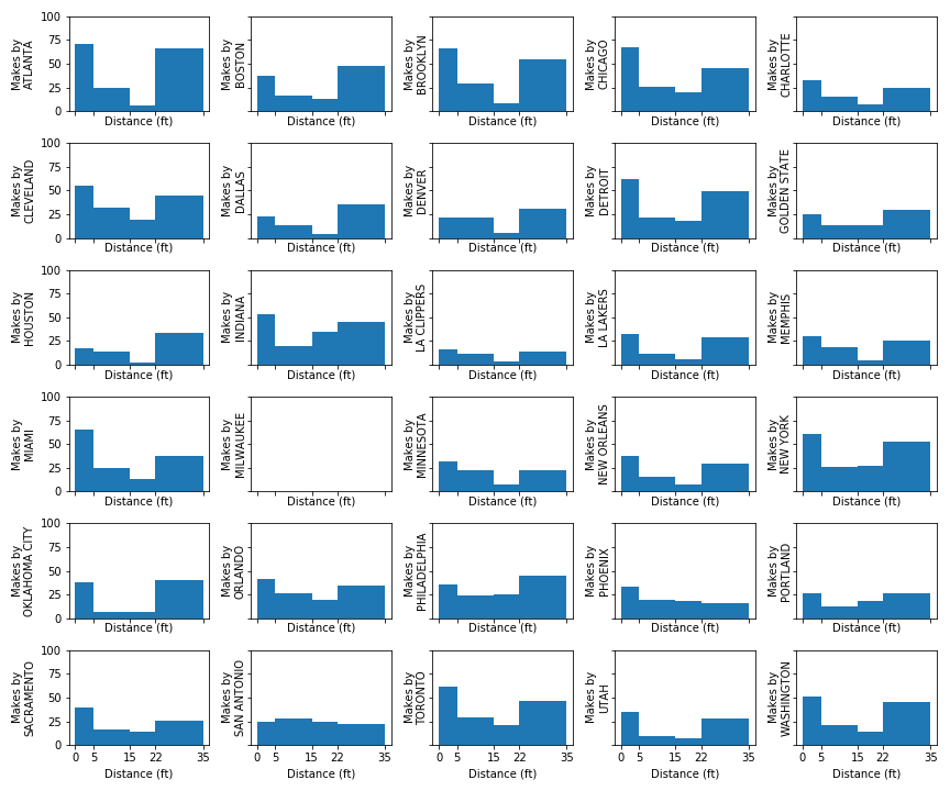
Comparing the worst defenses and best defenses (below), the best defenses allow very few short-range shots relative to allowing long-range shots. The worst defenses, however, seem to let a lot of layups and shots-in-the paint.
Cleveland’s Defense 18-19
Phoenix’s Defense 18-19
Atlanta’s Defense 18-19
Best NBA regular season defenses
Milwaukee’s Defense 18-19
Utah’s Defense 18-19
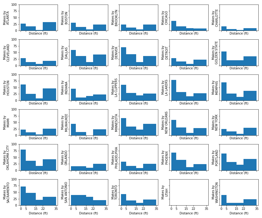
Indiana’s Defense 18-19
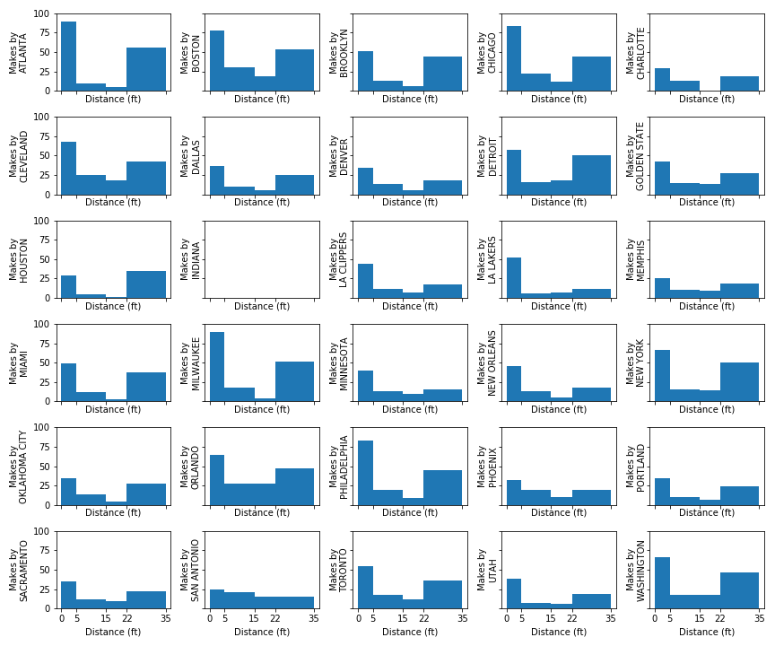
# Plotting a team's offense versus other teams
%matplotlib inline
import matplotlib.pyplot as plt
for column in df:
    fig, ax = plt.subplots(6,5, figsize=(12,10), sharex=True, sharey=True)

    for j, def_team in enumerate(df[column].index):
        row = j // 5
        col = j % 5
        ax[row, col].hist(df[column][def_team], bins=[0, 5, 15, 22, 35], density=False)
        ax[row,col].set_ylabel(f"Makes against\n{def_team}")
        ax[row,col].set_xlabel("Distance (ft)")
        ax[row,col].set_xticks([0, 5, 15, 22, 35])
        ax[row,col].set_xticklabels([0, 5, 15, 22, 35])
        ax[row,col].set_ylim([0, 100])

    fig.tight_layout()
    simple_name = '_'.join(a for a in column.split(' '))
    fig.savefig(f"{simple_name}_offense.png", transparent=True)
    plt.close(fig)
Worst NBA regular season offenses (by PPG)
Mempis’ Offense 18-19
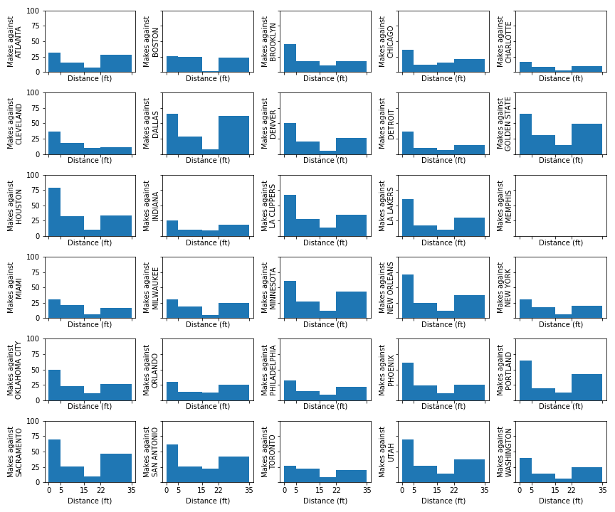
New York’s Offense 18-19
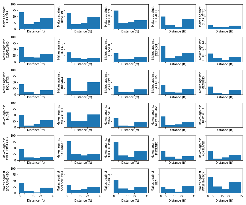
Cleveland’s Offense 18-19
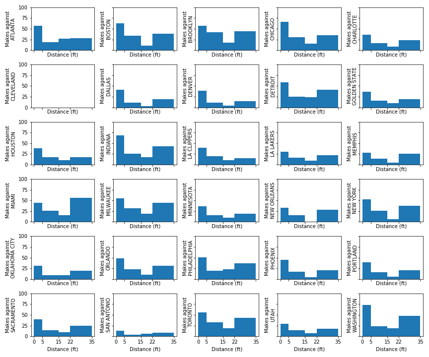
Best NBA regular season offenses (by PPG)
We can see Milwaukee and New Orleans’ offenses are very interior heavy, while Golden State has a relatively more balanced offense from all distances.
Milwaukee’s Offense 18-19
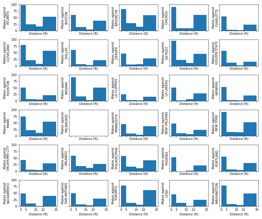
Golden State’s Offense 18-19
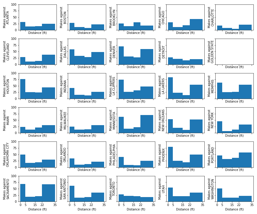
New Orleans’ Offense 18-19
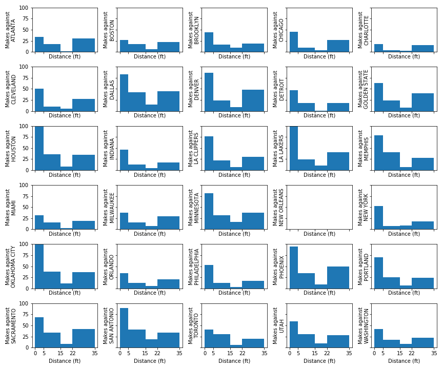
For a sanity check, Houston’s Offense 18-19
To make sure this method was “correct” we would expect Houston’s offense to be low in mid-range shots 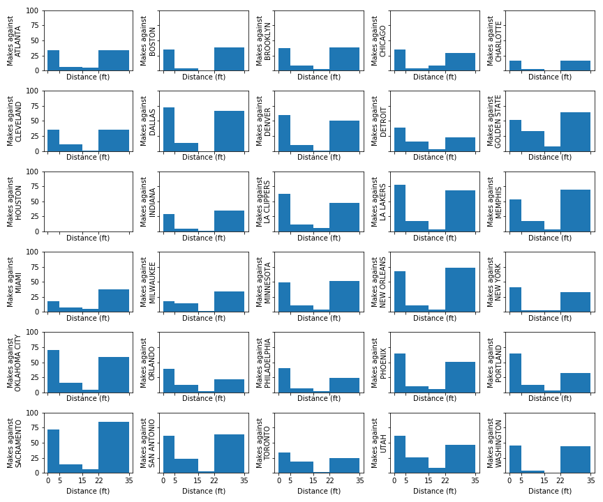
Room for improvement
Histogramming shot distances into 1 dimension of distance definitely misses essential locations like shots from the elbow, shots from the corner, top of the key, etc. 2D-histogramming, which is almost exactly like a shot chart, would make this analysis more robust to locations on the court. Along these lines, one could dissect this player-by-player, further simplifying to a player’s shot chart.
Alternatively, one could look at time left on the shot clock, shooter’s distance from nearest defender, the style of play involved (off-ball screen, pick and roll, post-up, etc.)
This notebook can be found here
