First-attempt at using PyMC3 for Bayesian parameter estimation

Applying some principles from earlier mcmc posts/notebooks to estimate the parameters of a linear model

import numpy as np
from numpy.random import random,rand
%matplotlib inline
import matplotlib
import matplotlib.pyplot as plt

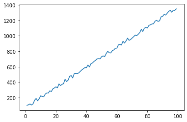
Generate some data, including some random noise

xvals = np.arange(1,100)
noise = rand(*xvals.shape)
yvals = 13*xvals + 50 + 50*noise

fig, ax = plt.subplots(1,1)
ax.plot(xvals, yvals)

[<matplotlib.lines.Line2D at 0x11989f518>]

from pymc3 import Normal, Uniform, Model, HalfCauchy

First pass at constructing a probability model. Our model is a line, but we need to describe the line’s parameters with distributions, and the parameters of the lines’ parameters’ distributions with distributions

For values that can be both negative and positive, we will use a Normal distribution, making up some wide-spread distributions. The centers of our slope and intercept distributions can be positive or negative

For values that can only be positive (like standard deviations), we will start out with a Uniform distribution

indices = [i for i,_ in enumerate(xvals)]
with Model() as my_model:
    # We have two parameters of interested, slope and intercept
    # We need to specify how we think the slope and intercept are distributed
    # Nested within that, there are parameters of those slope/intercept distributions
    # For those, we also need to specify how those parameters are distributed
    
    # Claims:
    # Our model is a line, y = ax + b
    # The slope follows a normal distribution
        # The center of this distribution is also normally distributed (m_a)
        # The sigma of this distribution is also normally distributed (s_a)
    # The intercept follows a normal distribution
        # The center of this distribution is also normally distributed (m_b)
        # The sigma of this distribution is also normally distributed (s_b)
    # The y-values (observed data) follow a normal distribution
        # The center of this distribution is based on our linear model guess
        # The sigma of this distribution is also normally distributed
    
    # We start with the leaves/root of the model, which is looking at the distributions
    # of the parameters that make up the slope/intercept distribution
    m_a = Normal('m_a', 10, sigma=10) # The slope's center is normally distributed
    m_b = Normal('m_b', 20, sigma=10) # The intercept's center is normally distributed
    # Second looking at the stdevs of the slope/center distributions
    s_a = Uniform('s_a', 10, 30) # The slope's stdev is uniformly distributed
    s_b = Uniform('s_b', 5, 15) # The intercept's stdev is uniformly distributed
    
    # With these parameters' distributions specified, we now build the distributions for 
    # the model's parameters
    a = Normal('a', m_a, sigma=s_a, shape=len(xvals)) # The slope's normal distribution
    b = Normal('b', m_b, sigma=s_b, shape=len(xvals)) # The intercept's normal distribution
    
    exp = a[indices]*xvals + b[indices]
    
    # Now let's look at our likelihood function (observed data distribution)
    s_y = Uniform('s_y', 30,50)
    #s_y = HalfCauchy('s_y', 1)
    y = Normal('y', exp, sigma=s_y, observed=yvals)

PyMC has some nice functionality to visualize which distributions and parameters feed into which other distributions and parameters. This was really helpful for me to understand the differences in the models, parameters, and distributions

from pymc3 import model_to_graphviz

model_to_graphviz(my_model)

Actually conduct the posterior sampling. Default uses a NUTS sampler. We use 2 different cores to independently run 2 different chains, with some guess starting values. 3000 samples was enough to get decent convergence, see note later

from pymc3 import sample

with my_model:
    my_trace = sample(3000, cores=2, start={'m_a':10, 'm_b':30})

Auto-assigning NUTS sampler...
Initializing NUTS using jitter+adapt_diag...
Multiprocess sampling (2 chains in 2 jobs)
NUTS: [s_y, b, a, s_b, s_a, m_b, m_a]
Sampling 2 chains: 100%|██████████| 7000/7000 [00:32<00:00, 109.64draws/s]
There were 68 divergences after tuning. Increase `target_accept` or reparameterize.
There were 78 divergences after tuning. Increase `target_accept` or reparameterize.
The acceptance probability does not match the target. It is 0.6827112736926122, but should be close to 0.8. Try to increase the number of tuning steps.
The estimated number of effective samples is smaller than 200 for some parameters.

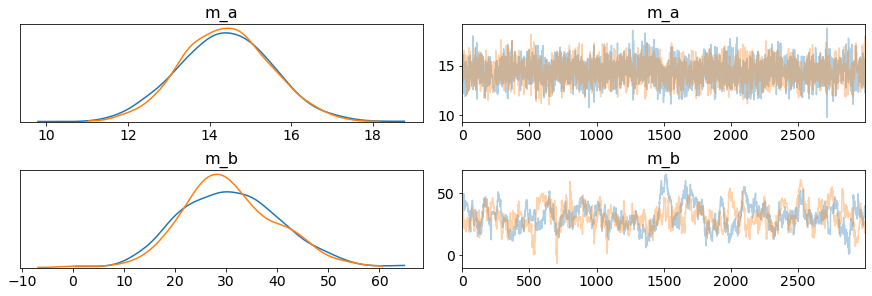
After sampling, we can visualize the trace which is the statistics equivalent of a molecular simulation trajectory. The top row plots the trace of the center of the slope distribution. There are a range of possibles slopes, here are their probabilities (on the left) and how the slope value was changed over the sampling. The bottom row plots the trace of the center of the intercept distribution.

The two 2 chains are both visualized for both parameters, and they converge decently, saying the chains ended up circulating through very similar values.

from arviz import from_pymc3, plot_trace

my_output = from_pymc3(my_trace)
plot_trace(my_output.posterior, var_names=['m_a', 'm_b']);

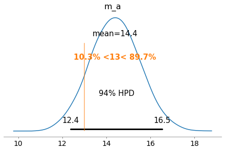
We can also plot the posterior distribution of the various parameters we sampled. In this case we will be looking at m_a which is the center of the normal distribution that models our slope.

We can also use these distributions to calculate probabilities of observing certain slopes. In this case, we can look at the true slope (that we specified), and see it’s 89.7% more likely to observe a slope greater than 13. This doesn’t seem very promising for our probability model, if it says a slope of 13 isn’t very likely

from arviz import plot_posterior

plot_posterior(my_trace, var_names=['m_a'], ref_val=13)

array([<matplotlib.axes._subplots.AxesSubplot object at 0x1c2e53f898>],
      dtype=object)

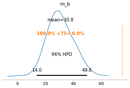
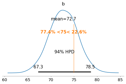
We can apply the same function to look at the center of the distribution that represents the intercept of our line. Originally, we specified it as 50 + 50 *noise, which means the intercept would vary from [50, 100)

Interestingly, it is VERY likely to observe an intercept less than 75. Given our random noise, you’d expect the intercept to be ~75, but the bayesian probability model would suggest otherwise.

If we look at both slope and intercept, the slope is over-predicted and intercept under-predicted, where each correction compensates for the other parameter

plot_posterior(my_trace, var_names=['m_b'], ref_val=75)

array([<matplotlib.axes._subplots.AxesSubplot object at 0x1c2f8d3c18>],
      dtype=object)

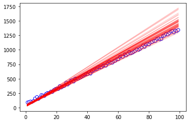
So our slope is overestimated and intercept underestimated - how does the line actually look?

We can plot the observed data as the empty circles, and pick a couple parameters from our trace to make a new line. We’re pulling randomly from the last 200-ish of the sampling, some sort of steady-state sampling region, and pulling from chain 1.

So this visually shows that our slope is overestimated and intercept underestimated - this is not good

fig, ax = plt.subplots(1,1)
ax.plot(xvals, yvals, color='b', marker='o', markerfacecolor='white')
for i in range(50):
    random_idx = np.random.randint(800,1000)
    slope = my_output.posterior.m_a[1][random_idx].values
    intercept = my_output.posterior.m_b[1][random_idx].values
    ax.plot(xvals, slope*xvals + intercept, color='red', alpha=0.2)

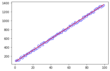
For comparison, we can do a plain linear regression to fit the data.

With this method, it’s not as simple to look at various probabilities of slopes or distributions of parameters. The number is the number you get from fitting the data, a singular value.

We can report correlation coefficients to get an idea of how good of a model it is, but we don’t get a sense of the distribution of the slopes/intercepts.

But with the linear regression, the fit is much better. The slopes and intercepts are more in line with what we’d have expected from making up the data.

from sklearn.linear_model import LinearRegression
xvals = xvals.reshape(-1,1)
yvals = yvals.reshape(-1,1)
reg = LinearRegression().fit(xvals, yvals)
print(reg.score(xvals, yvals))
print((reg.coef_, reg.intercept_))

0.998515144087584
(array([[13.01389575]]), array([73.01098003]))

fig, ax = plt.subplots(1,1)
ax.plot(xvals, yvals, color='b', marker='o', markerfacecolor='white')
ax.plot(xvals, xvals*reg.coef_ + reg.intercept_, color='r')

[<matplotlib.lines.Line2D at 0x1c2f715358>]

Can we do better with the Bayesian model? Let’s simplify a little. Before we were modeling slope and intercept with a normal distribution, but the normal distribution’s parameters were unknown - we were sampling parameters of those normal distribution, which will propagate up to the actual slopes.

Instead, let’s just have “fixed” parameters to represent the normal distributions. This sort of “constrains” what we have since we’ve already made a claim on the distributions of a and b, without having a distribution on the distribution of a and b. On the bright side, this reduces the degrees of freedom or room for error in the sampling.

As in the examples from the mcmc notebook 4, they chose to use a Half Cauchy distribution for their standard deviations (this distribution enforces only positive values, so that’s good for standard deivation). Looking at some stack exchange responses, half-Cauchy can be weakly-informative, which helps if the posterior distribution is the more-dominant factor. For generally choosing priors, it depends on what the prior beliefs are and if you can fit them to some of the more common distributions or your own intuitive understanding.

indices = [i for i,_ in enumerate(xvals)]
with Model() as half_cauchy_model:
    # Claims:
    # Our model is a line, y = ax + b
    # The slope follows a normal distribution (a)
    # The intercept follows a normal distribution (b)
    # The y-values (observed data) follow a normal distribution
        # The center of this distribution is based on our linear model guess
        # The sigma of this distribution is also distributed by half-cauchy
   
    
    # We now build the distributions for 
    # the model's parameters
 
    a = Normal('a', 13, sigma=20)
    b = Normal('b', 60, sigma=20)
    
    exp = a*xvals + b
    
    # Now let's look at our likelihood function (observed data distribution)
    s_y = HalfCauchy('s_y', beta=10, testval=1)
    y = Normal('y', exp, sigma=s_y, observed=yvals)

Visualizing the simplified model, with a smaller hierarchy

from pymc3 import model_to_graphviz

model_to_graphviz(half_cauchy_model)

from pymc3 import sample

with half_cauchy_model:
    half_cauchy_trace = sample(3000, cores=2, start={'a':10, 'b':50})

Auto-assigning NUTS sampler...
Initializing NUTS using jitter+adapt_diag...
Multiprocess sampling (2 chains in 2 jobs)
NUTS: [s_y, b, a]
Sampling 2 chains: 100%|██████████| 7000/7000 [00:08<00:00, 787.34draws/s]
The acceptance probability does not match the target. It is 0.8871159685668408, but should be close to 0.8. Try to increase the number of tuning steps.

from arviz import from_pymc3, plot_trace

half_cauchy_output = from_pymc3(half_cauchy_trace)
plot_trace(half_cauchy_output.posterior, var_names=['a', 'b']);

plot_posterior(half_cauchy_trace, var_names=['a'], ref_val=13)

array([<matplotlib.axes._subplots.AxesSubplot object at 0x1c2b871828>],
      dtype=object)

plot_posterior(half_cauchy_trace, var_names=['b'], ref_val=75)

array([<matplotlib.axes._subplots.AxesSubplot object at 0x1c345d8940>],
      dtype=object)

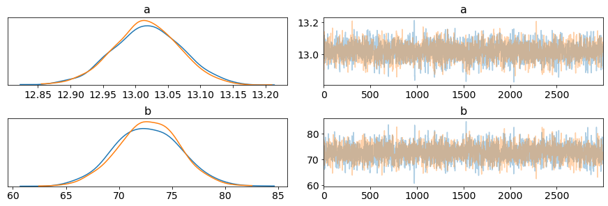
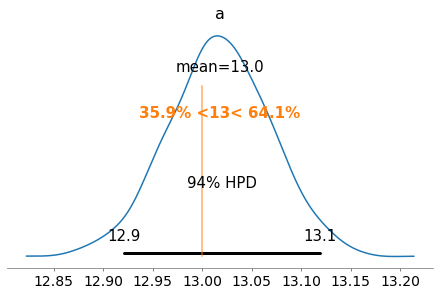
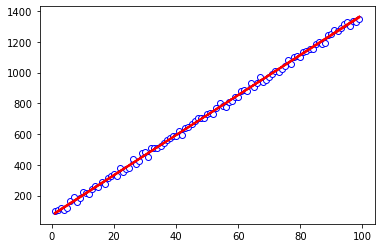
Visualizing all the traces (which converge well with each other) and posteriors, the distributions all aggregate around correct centers/locations. Actually visualizing some of the resultant lines, the lines fit much more nicely than before.

fig, ax = plt.subplots(1,1)
ax.plot(xvals, yvals, color='b', marker='o', markerfacecolor='white')
for i in range(50):
    random_idx = np.random.randint(800,1000)
    slope = half_cauchy_output.posterior.a[1][random_idx].values
    intercept = half_cauchy_output.posterior.b[1][random_idx].values
    ax.plot(xvals, slope*xvals + intercept, color='red', alpha=0.2)

Summary

This was my first-hand pass of using Bayesian parameter estimation to estimate the slope and intercept of an analytically-specified line (with some noise). I tried to ‘chain priors’ together by using distributions to esimate the parameters that described the distributions of the slope/intercept, but the estimated paramters were poor. I simplified the model to “hard code” the distribution underlying the slope and intercept and got much better results. Still, the sklearn linear regression still had pretty good slope/intercept estimates, but the Bayesian methods were able to provide insight on the distribution/range of parameters that could model the line - even if some were worse than others.

As in MD, sampling is always important (did you sample enough space, did you sample long enough, did doing multiple trials converge on the same trace/trajectory?) I think, when chaining priors together, we were doing a more thorough sampling through phase space, which led to worse convergence and a wilder range of parameter estimates (compare the x-scales of some of these plots for the parameter estimates). Without chaining priors, we were searching through space less and converged a litle more easily. As with most computational methods, it’s important to choose the approach that is most appropriate for your task - there is never a silver bullet.