Conducting a simulation

Running a simulation means taking a model and sampling sort of distribution with it.

Note: Simulation was built using mBuild and foyer, simulated using HOOMD-blue

Recapping molecular modeling

Remember, our model from a molecular modeling perspective is the potential energy, which depends on the coordinates of every atom or particle in the system. We can either model the system energy using QM or MM methods. QM methods are more accurate, but more expensive. MM methods simplify away some of the less-relevant details (this depends on your system), make some approximations, and allow us to study larger and slower systems.

The Boltzmann distribution

The Boltzmann distribution describes the probability of observing states as a function of its energy and other thermodynamic variables (like the temperature). Delving into the thermodynamic theory, the Boltzmann distribution is the distribution that maximizes a system’s entropy, so this is a physically-rooted distribution. Concisely put into an equation:

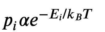
where $p_i$ is the probability of a state, $E$ is the energy of that state, $k_b$ is Boltzmann’s constant, and $T$ is the temperature

What is a ‘state’?

In the Boltmzann distribution, a state refers to an energetic state (which can be associated to a chemical structure’s 3D coordinates. Going further, depending on our thermodynamic conditions, we have macrostates that desribe a system’s macroscopic properties (like temperature, pressure, volume, energy, number of particles). There are a set of microstates that can satisfy or achieve a particular macrostate.

For example, if you had 3 coins, you could have a macrostate consisting of 2 Tails and 1 Head. The corresponding microstates might be HTT, THT, TTH

Application to molecular simulation

One often overlooked fact is that all molecules move around, a lot or a little (unless you’re at absolute zero but that’s not the point). Thermal motion means that every atom vibrates a little bit - every molecule can wiggle ever so slightly or fly around. However, the physical phenomenon that atoms move around is the whole reason we have a distribution of configurations (coordinates)

Under the Boltzmann distribution, the probability of witnessing a chemical microstate (a particular set of coordinates that a chemical configuration occupies) is related to the energy of that state.

If a particular configuration is high-energy, we probably won’t witness it. If it low-energy, there is a good chance we will

Monte Carlo methods

Monte carlo (MC) sampling is not unique to molecular simulation, but molecular modelers do like to implement MC methods.

Briefly, MC methods involve a trial where you try to change/alter some part of your system. In molecular modeling, your MC trial moves involve altering your configuration (rotating a molecule, displacing an atom, stretching a bond, etc.)

The choice to accept this move depends on the energy before and after the trial move. If the energy is lower, we accept the move and proceed with the simulation. If the energy is higher, we calculate the relative probabilities (according to the Boltzmann distribution), and compare that to a randomly-generated number; we either reject the move and propose a new one or accept and proceed.

There are lots of different algorithms, but a common one in the molecular modeling field is the Metropolis-Hastings algorithm

If you sample a lot of configurations, you can eventually get a good idea of the distribution of various configurations of your system. From this resultant sample or trajectory, we can start computing various (static) properties. By nature of the sampling, the configurations are somewhat independent and uncorrelated compared to other sampling methods

Molecular dynamics methods

In molecular dynamics (MD) sampling, we utilize kinetic energy and momentum to actually simulate the motion of these atoms. This is where we bring Newton’s laws of motion in order to physically capture these motions - the acceleration on an object is related to the forces acting upon it

To compute the forces acting upon each atom, we look back to another physical relationship - force is the negative derivative of energy with respect to distance. This works well because now we we can relate motion to our molecular model; given the energy of our system, compute the gradient to get the forces, and these forces dictate the acceleration

There a variety of other formalisms that have been used in MD like Hamiltonian or Lagrangian mechanics, but the idea is to relate potential and kinetic energy to the motion of a system

We also know that

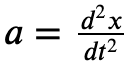
Which means we can relate acceleration to position via a second order ordinary differential equation. If we integrate this, we can get a system’s position over time.

This is very hard to do analytically, so we often resort to various numerical methods to integrate a second order ODE (compute the gradient and take a small step in that direction). In MD, we call this an integrator, and the field is very interested in all the different integration algorithms, their computational complexity, and overall stability (energy conservation versus time step, time-reversibility, among others). Don’t forget, this integration means we now also account for things like velocity and kinetic energy (which follow the Maxwell-Boltzmann distribution)

To summarize molecular dynamics, we are integrating Newton’s equations of motion over time according to a potential energy function.

After integrating for a finite number of steps, we have sampled a number of configurations that are more correlated to each other compared to MC methods.

Statistical side note

As a molecular modeler venturing into broader areas of statistics and data science, I find myself trying to relate concepts like Markov chain Monte Carlo or Hamiltonian dynamics back to these molecular modeling notions of MC and MD. I think there are similarities in that the MC analogs are drawing random samples, but the Hamiltonian and MD methods are accounting for some sort of kinetics or momentum. Even the notion of some steepest descent gradient algorithms reminds me that we essentially compute a gradient (force) of our objecive function (energy).

The law of large numbers, ergodicity, and phase space

As in statistics, the only way we can reliably trust our sample is if we draw enough samples. If we sample enough, the sample statistics and population statistics relate well.

In simulation, before we can even begin to think about drawing enough samples, we have to draw physically correct samples. We call this ergodicity - when our the probability distributions from our simulations don’t change much. This means we need to run a simulation long enough such that our sampled configurations results replicate the underlying physical distributions.

Here’s a more involved discussion. For N atoms, we have 6 N variables (for the 3 dimensions we have a velocity/momentum and a position). This results in a 6N phase space. Over the course of the simulation, we are effectively traversing through 6N phase space, with some regions being more “popular” or favorable than others. When this probability density no longer changes with respect to time, our system is ergodic and we just need to generate a lot of samples from this probability distribution.

The formulation (Liouville’s theorem) is as follows

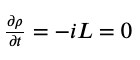
A simpler way of thinking about this: you can start a simulation from some very unrealistic coordinates (like water in a crystalline configuration even though you’re at room temperature), but if you simulate long enough, eventually you begin visiting only the physically-realistic and probabilistic configurations. At this point, your system is equilibrated and then you begin the task of sampling from this distribution. So if you run a 100 ns simulation, you might discard the first 20 ns as “burn-in” or “equilibration” when you were trying to hit equilibration. The other 80 ns you actually care about and analyze - this is your “production” run where you are reliably sampling from the correct distribution (also considered steady-state).

MC vs MD

There are a variety of things to think about here: computational complexity, equilibration, and the physical properties you want to measure. But at the end of each simulation, you end up with a series of configurations (coordinates).

Computational complexity

In most force fields (potential energy functions), bonded interactions are cheap because each atom participates in maybe a dozen different bonded interactions. Nonbonded interactions are much harder becuase each atom participates in a nonbonded interaction with every other atom in your system, this is $O(n^2)$, and these nonbonded, pairwise interactions are the most expensive calculations in a simulation code. In reality, there are some simulation tricks to speed up this pairwise computation to only look at the relevant/nearby atoms (neighbor lists) or use reciprocal space to rapidly compute long-distance interactions (Ewald sums)

In MC, you don’t move EVERY atom, you move a few or just one. To evaluate a trial move, you need to compute how the energy changes. Fortunately, for the 99% of atoms that didn’t move, that saves you some energy calculations. You only need to calculate the energy for the part of the system that changed.

In MD, you are moving EVERY atom, so you have to do this $O(n^2)$ calculation every, single time.

So comparing each iteration, a single MC iteration is faster than a single MD iteration. Actually, for various reasons, MD algorithms have found success being implemented as GPU kernels, so MD is really accelerated by GPUs. The complexity of MC has inhibited MC packages from really harnessing the computational power of a GPU. Don’t get me wrong, there are some MC packages that utilize the GPU fantastically well, but you can find more MD packages that use the GPU.

Equilibration

MC means we take “random” moves - we could twist a long polymer, move an atom halfway across the simulation box, or something creative. Because MD aims to simulate the motion of atoms, our moves are somewhat constrained to local displacements.

With a wider variety, and more “radical” moves, MC can reach equilibration faster than MD, whose moves are very dependent on small displacements

Physical properties

It’s 2-0, so we have to find something in favor of MD. Some physical properties depend on the time-evolved-dynamics of a system - we care about how the coordinates relate to each other over time. MC cannot do this because each configuration is fairly uncorrelated from the previous one. In MD, these configurational correlations help us calculate transport properties like viscosity and diffusion. MC has a hard time computing these properties due to the lack of correlation between configurations

A grad student confession

Honestly, most comptuational grad students don’t think about these underlying theories or formulations that often. We’re more concerned with applying them to do our research. We often take coursework that covers these concepts, but more often than not, we shrug off simulation techniques as just calculating energy/forces and moving atoms.

In terms of implementing these algorithms, they are already well-implemented in existing software packages. We don’t have to write our Metropolis-Hastings algorithms, MC moves, or integrators - other generations of academics, scientists, and engineers have constructed and tested these tools and made sure they work. They made way for newer generations of students to spend their time applying these tools to research.

Usually, a particular lab or field gravtitates to either MC or MD, and then that becomes the learning environment and code infrastructure for new students. Occasionally we move into another method, but only if the scientific problem truly necessitates using another method.

Should the (unfortunate) time come when we have to find bugs in these packages, then we dust off the textbooks and re-re-re-re-learn these algorithms and techniques.

Conclusion

There are a variety of simulation/sampling techniques (MD or MC), each with its own perks and drawbacks. Fundamentally, there is a lot of derivation and proof that validates these methods in sampling the Boltzmann distribution. The tools of other scientists and engineers have allowed us to study interesting scientific problems without being “caught in the weeds”.

In broader statistical/data science perspectives, we use simulation methods to sample from a distribution and compute various properties (some dependent on time-correlations), and we have to ensure that we have correctly sampled enough to draw reliable conclusions. Some build the model and simulation cornerstones, others apply these tools as they see fit.